Getting Started with Linear Regression

With Mlektic, you can perform univariate or multivariate linear regression using the least squares method or by considering various optimization options available in the optimizer_archt module.

Supported optimization methods include: - ‘sgd-standard’ - ‘sgd-stochastic’ - ‘sgd-mini-batch’ - ‘sgd-momentum’ - ‘nesterov’ - ‘adagrad’ - ‘adadelta’ - ‘rmsprop’ - ‘adam’ - ‘adamax’ - ‘nadam’

For more details on the optimizer_archt module, please refer to the optimizer_archt documentation.

You can also apply regularization to improve model generalization. The regularizer_archt module supports the following regularization methods: - ‘l1’ (default) - ‘l2’ - ‘elastic_net’

To learn more about the regularizer_archt module, please refer to the regularizer_archt documentation.

For example, you can train a model using linear regression with standard gradient descent and L1 regularization with the LinearRegressionArcht module as follows:

from mlektic.linear_reg import LinearRegressionArcht
from mlektic import preprocessing
from mlektic import methods
import pandas as pd
import numpy as np

# Generate random data.
np.random.seed(42)
n_samples = 100
feature1 = np.random.rand(n_samples)
feature2 = np.random.rand(n_samples)
target = 3 * feature1 + 5 * feature2 + np.random.randn(n_samples) * 0.5

# Create pandas dataframe from the data.
df = pd.DataFrame({
    'feature1': feature1,
    'feature2': feature2,
    'target': target
})

# Create train and test sets.
train_set, test_set = preprocessing.pd_dataset(df, ['feature1', 'feature2'], 'target', 0.8)

# Define regularizer and optimizer.
regularizer = methods.regularizer_archt('l1', lambda_value=0.01)
optimizer = methods.optimizer_archt('sgd-standard')

# Configure the model.
lin_reg = LinearRegressionArcht(iterations=50, optimizer=optimizer, regularizer=regularizer)

# Train the model.
lin_reg.train(train_set)

Epoch 5, Loss: 15.191523551940918
Epoch 10, Loss: 11.642797470092773
Epoch 15, Loss: 9.021803855895996
Epoch 20, Loss: 7.08500862121582
Epoch 25, Loss: 5.652813911437988
Epoch 30, Loss: 4.592779636383057
Epoch 35, Loss: 3.807236909866333
Epoch 40, Loss: 3.2241621017456055
Epoch 45, Loss: 2.790440320968628
Epoch 50, Loss: 2.4669017791748047

To learn more about the LinearRegressionArcht module, please refer to the LinearRegressionArcht documentation.

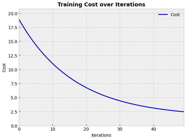
The cost evolution can be plotted with the plot_cost method:

from mlektic.plot_utils import plot_cost

cost_history = lin_reg.get_cost_history()
plot_cost(cost_history, dim=(7, 5))

cost plot

Different evaluation metrics can be obtained:

mse = lin_reg.eval(test_set, 'mse')
rmse = lin_reg.eval(test_set, 'rmse')
mae = lin_reg.eval(test_set, 'mae')
mape = lin_reg.eval(test_set, 'mape')
r2 = lin_reg.eval(test_set, 'r2')
corr = lin_reg.eval(test_set, 'corr')

print(f'MSE: {mse}')
print(f'RMSE: {rmse}')
print(f'MAE: {mae}')
print(f'MAPE: {mape}')
print(f'R²: {r2}')
print(f'Coeficiente de Pearson: {corr}')

MSE: 2.451315402984619
RMSE: 1.565667748451233
MAE: 1.28024423122406
MAPE: 38.169368743896484
R²: 0.3232208490371704
Coeficiente de Pearson: 0.9599050283432007

Print the parameters obtained by training:

print("Weights:", lin_reg.get_parameters())
print("Intercept:", lin_reg.get_intercept())

Weights: [[1.0966599]
[1.3730361]]
Intercept: [1.9968479]

And make predictions:

prediction = lin_reg.predict(2.0)
print(f'Prediction: {prediction[0][0]}')

Prediction: 6.936239719390869

Finally, you can save the model parameters in a JSON format for future use:

lin_reg.save_model('linear_regression_model.json')